Background
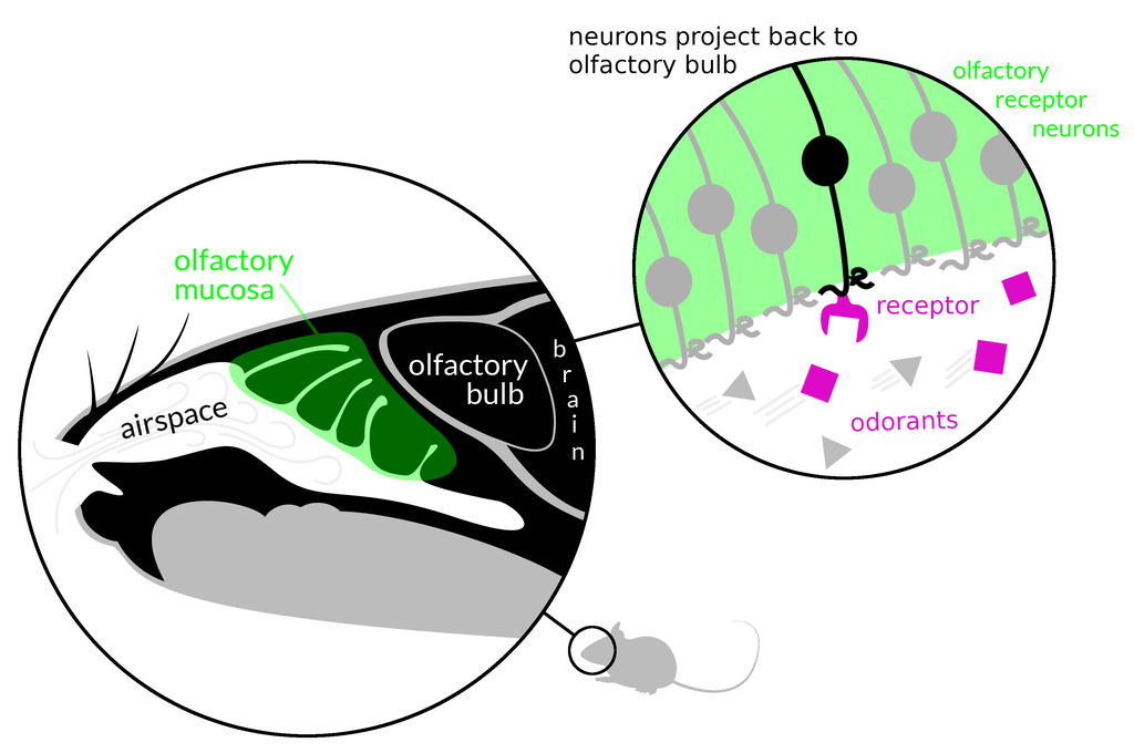
Olfactory sensory neurons, resident to the olfactory epithelium of the nose, bind directly to odorant (scent
) molecules in the air and transmit a signal to the brain in response. To rough approximation, each of these neurons expresses only one or several types of receptor of several hundred (nearly 400 in humans, and more than 1000 in mice), and thus binds with greatest affinity to only one or a few odorants. The electroolfactogram (EOG), recorded at the surface of the olfactory epithelium, is the electrical potential generated across a field of olfactory sensory neurons in response to this binding, evoked upon the presentation of an olfactory stimulus (i.e. scent). As intact signal transduction machinery (present in mature olfactory neurons) is requisite for the presence of EOG signal, and as its dynamics are indicative of the health of the local cell niche, the EOG is a useful functional assay of olfaction at the level of the epithelium.
Justification
I am designing the μEOG (micro-Electroolfactogram) as a compact and low cost device to replace the myriad of bulky and expensive equipment1 (costing on the order of thousands or tens of thousands of dollars) traditionally used for the recording of EOGs from olfactory tissue in a laboratory setting. I aim to create a cheap, precise, mains-isolated, highly noise-resistant biopotential recording system, designed for stimulating and measuring EOGs (but flexible enough to measure other biopotentials with little to no modification), and to make the plans and software freely available for others to use or modify. The conventional EOG monitoring rig consists of a separate amplifier, digitizer, compressed air tank (or two), regulators, and pressurized pulse delivery apparatus, along with a computer (for data collection and experiment control) and other supporting equipment. In this setup, a pulled-glass pipette electrode (containing a chlorided silver wire and electrolyte solution) is gently placed atop a dissected piece of olfactory tissue (a second chlorided silver wire, acting as signal ground, is electrically connected to the tissue by way of the electrolyte solution upon which the tissue rests), and a humidified low pressure, 'high' flow rate (~600 mL/min) odorant-free air stream is aimed across the top of the tissue. Here, absent of a specific olfactory stimulus, a baseline signal is measured. Into the air stream, a 100 ms-long, 10 psi puff of concentrated odorant (e.g. amyl acetate, which smells like bananas) is injected, and the electrical response of the tissue to this olfactory stimulus is measured.
Improvements & Implementation
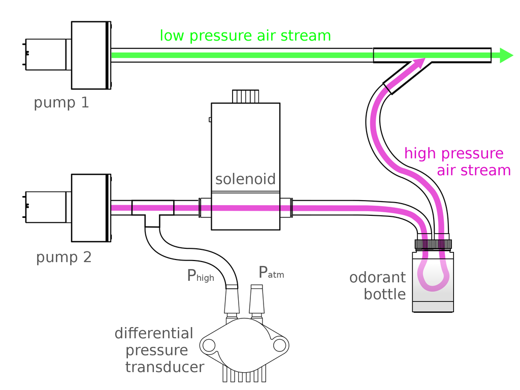
A large fraction of this setup is dedicated to compressed-air handling; including one or more compressed air tanks (responsible for providing the low and high pressure air streams), multiple regulators, and specialized pressurized air pulse delivery equipment. The μEOG is designed to sidestep this requirement. In the μEOG, these will be replaced with two small diaphragm pumps (like those used to inflate portable automated blood-pressure cuffs): one for the low pressure stream and one for the high pressure pulses. To deliver the high pressure pulses, one of the diaphragm pumps will be pumped against a closed (normally closed) solenoid valve until the pressure (as monitored by a pressure transducer) reaches 10 psi, as compared to atmospheric pressure. At this point, the solenoid valve will be opened for the pulse duration (100 ms by default), and then closed. Pressure will be monitored during this pulse and maintained at 10 psi, though for pulse durations on the order of 100 ms, significant adjustments to the pressure are not likely to be required.
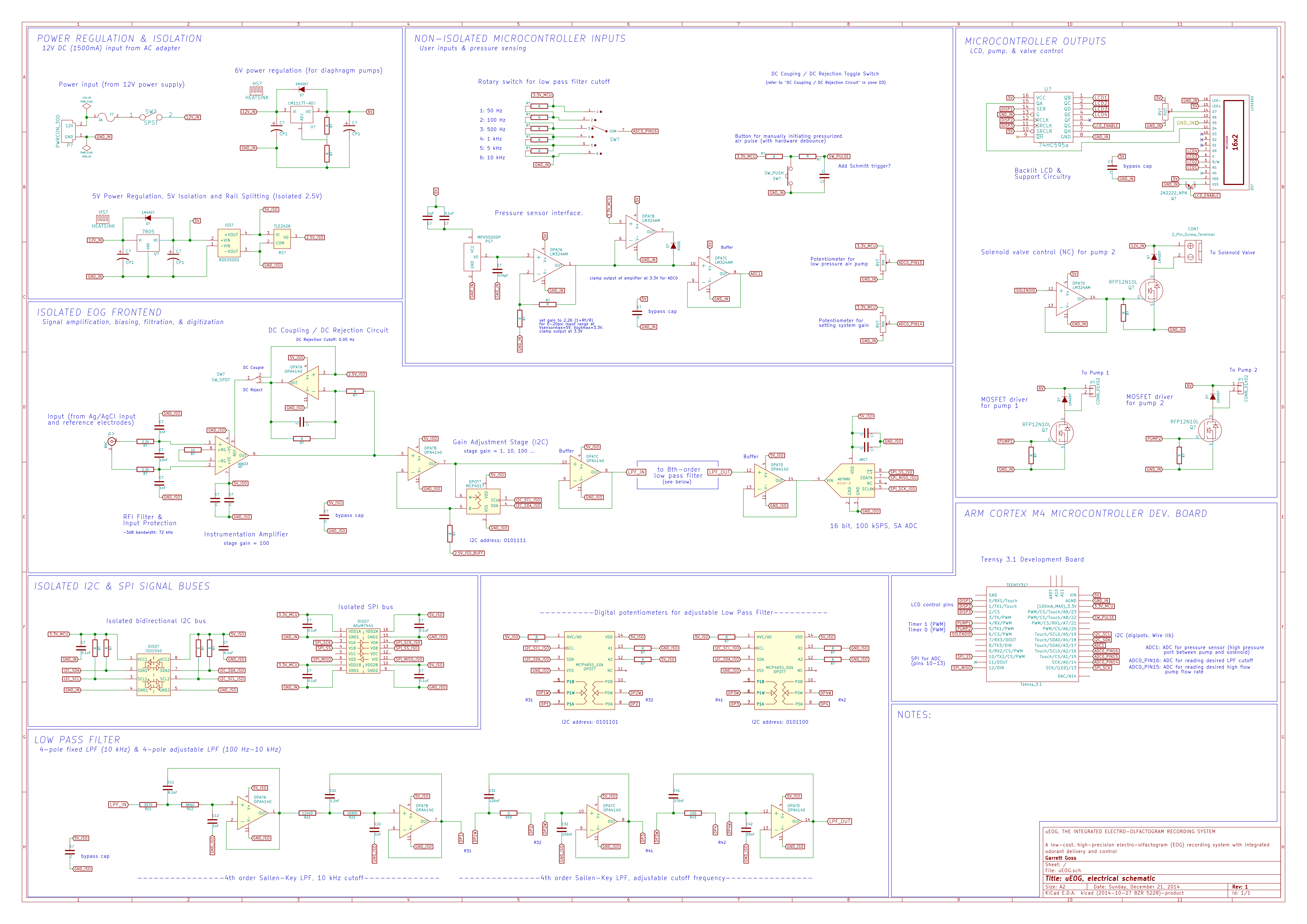
The pumps, air pressure and flow rate control, and all other functions of the setup (including the biopotential amplification, analog filtration, isolation, digitization, and control), will be integrated into a single device, small enough to fit within a 8x 7
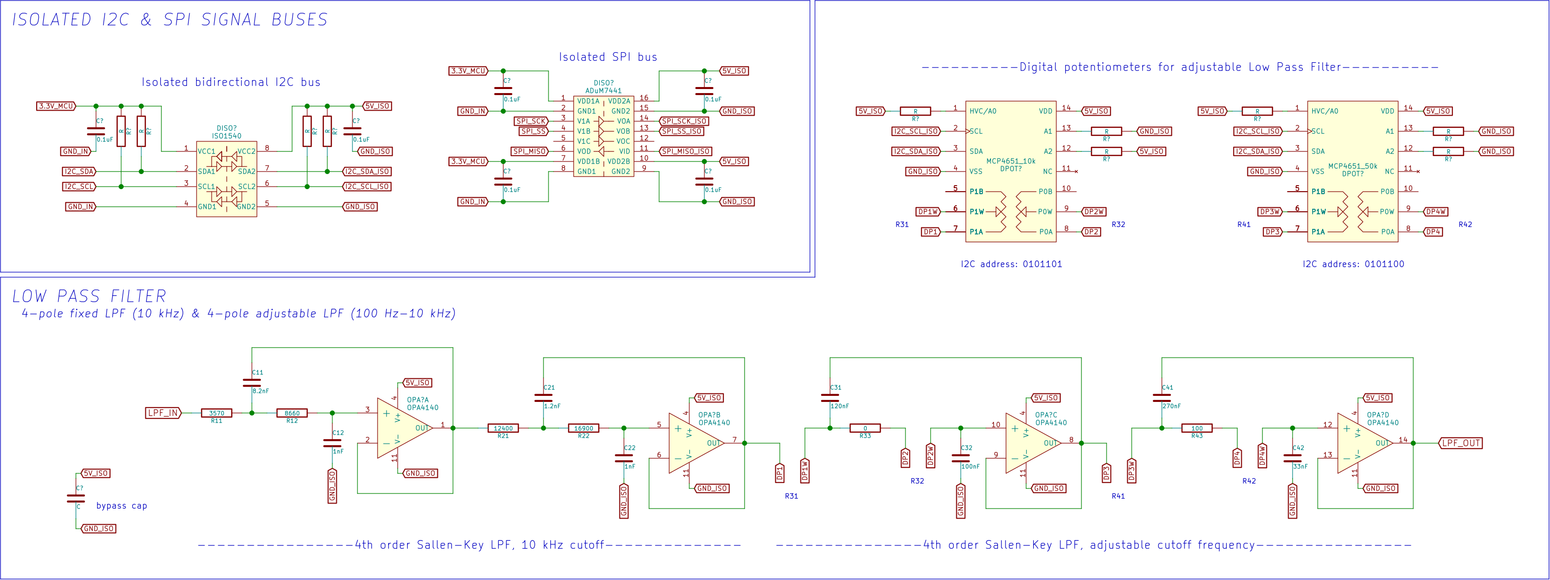
x 2.5" enclosure. Device status will be displayed on an LCD on the front of the device, and settings will be adjustable via dedicated rotary switches, potentiometers, and buttons, and via software on a PC connected for data collection. Processing and control of inputs and outputs will be performed by a Teensy 3.1 development board, based on an Freescale ARM Cortex M4 microcontroller (MK20DX256VLH7). Input from the electrodes (run from tissue to device as a shielded twisted-pair) will be passed through a passive RFI-rejection filter (-3 dB bandwidth of 72 kHz) and into an AD623 instrumentation amplifier (in-amp), differentially, with gain set to 100. The REF pin of the in-amp will either be connected to the isolated 2.5 V rail (provided by a TLE2426 rail-splitter, itself supplied by an ROE0505s isolated 5 V-input/5 V-output DC-DC converter) to DC couple the input to the center of the 5 V working range of the ADC, or to the output of an inverted, 0.05 Hz low pass filtered, 2.5 V offset version of the in amp output for DC-rejection (i.e. any components below 0.05 Hz will be subtracted from the signal, rejecting drift due to very low frequency components of the input, or due to DC drift created by RFI noise aliasing in the in-amp). Next, the signal is passed to a digitally adjustable gain stage (gain controlled by digital potentiometer, or digipot) and buffer, to an active fixed-cutoff 4th-order 10 kHz-cutoff Butterworth (Sallen-Key) low pass filter (LPF), an active, digitally-controlled adjustable-cutoff 4th-order Butterworth LPF, and finally to another buffer before being digitized by an external 16 bit, 100 kSPS serial-approximation ADC (Analog Devices AD7680). The output of this is carried over an isolated SPI bus (Analog Devices ADuM7441) to the microcontroller. The cutoff frequency of the 4-pole adjustable LPF is adjusted by changing the resistance of the 4 digipots (2 x dual 256-position Microchip MCP4651) used within two cascaded 2-pole Sallen-Key LPF stages, optimized to closely match ideal 4th-order Butterworth filter parameters using MATLAB, signaling these changes over an isolated I2C bus (Texas Instruments ISO1540).
MATLAB Filter Optimization
First, let's define a few functions that will be useful later on:
SKB_LPF_generic.m
function output = SKB_LPF_generic(fc,poles)
% SKB_LPF_GENERIC Creates the transfer function of a 2, 4, 6, or 8-pole
% Butterworth low pass filter with a given -3dB cutoff frequency, built
% from 2-pole filter stages.
%
% Returns a structure array containing:
%
% - vectors of the coefficients (ordered by descending power of s)
%   of the numerator and denominator of the transfer function of each
%   2-pole stage,
%
% - vectors of the coefficients of the numerator and denominator of the
%   transfer function of the filter as a whole (from the cascaded 2-pole
%   stages), and
%
% - the continuous-time transfer function of the entire filter.
%
% OUTPUT = SKB_LPF_GENERIC(fc,poles)
%
% OUTPUT.n1 ... OUTPUT.n4   numerator coefficients of individual stages
% OUTPUT.d1 ... OUTPUT.d4   denominator coefficients of individual stages
% OUTPUT.n                  numerator coefficients of whole filter
%                           transfer function
% OUTPUT.d                  denominator coefficients of whole filter
%                           transfer function
% OUTPUT.cascade            complete continuous-time transfer function
%

switch poles
    case 2
        Q = [0.7071];
        output.n1 = (2*pi*fc)^2;
        output.d1 = [1 2*damping_ratio(Q(1))*(2*pi*fc) (2*pi*fc)^2];
        output.n = output.n1;
        output.d = output.d1;
        output.cascade = tf([output.n],[output.d]);
    case 4
        Q = [0.5412 1.3065];
        output.n1 = (2*pi*fc)^2;
        output.d1 = [1 2*damping_ratio(Q(1))*(2*pi*fc) (2*pi*fc)^2];
        output.n2 = output.n1;
        output.d2 = [1 2*damping_ratio(Q(2))*(2*pi*fc) (2*pi*fc)^2];
        output.n = multpolys(output.n1,output.n2);
        output.d = multpolys(output.d1,output.d2);
        output.cascade = tf([output.n],[output.d]);
    case 6
        Q = [0.5177 0.7071 1.9320];
        output.n1 = (2*pi*fc)^2;
        output.d1 = [1 2*damping_ratio(Q(1))*(2*pi*fc) (2*pi*fc)^2];
        output.n2 = output.n1;
        output.d2 = [1 2*damping_ratio(Q(2))*(2*pi*fc) (2*pi*fc)^2];
        output.n3 = output.n1;
        output.d3 = [1 2*damping_ratio(Q(3))*(2*pi*fc) (2*pi*fc)^2];
        output.n = multpolys(output.n1,output.n2,output.n3);
        output.d = multpolys(output.d1,output.d2,output.d3);
        output.cascade = tf([output.n],[output.d]);
    case 8
        Q = [0.5098 0.6013 0.8999 2.5628];
        output.n1 = (2*pi*fc)^2;
        output.d1 = [1 2*damping_ratio(Q(1))*(2*pi*fc) (2*pi*fc)^2];
        output.n2 = output.n1;
        output.d2 = [1 2*damping_ratio(Q(2))*(2*pi*fc) (2*pi*fc)^2];
        output.n3 = output.n1;
        output.d3 = [1 2*damping_ratio(Q(3))*(2*pi*fc) (2*pi*fc)^2];
        output.n4 = output.n1;
        output.d4 = [1 2*damping_ratio(Q(4))*(2*pi*fc) (2*pi*fc)^2];
        output.n = multpolys(output.n1,output.n2,output.n3,output.n4);
        output.d = multpolys(output.d1,output.d2,output.d3,output.d4);
        output.cascade = tf([output.n],[output.d]);``
    otherwise
        disp('Please enter an even number of poles between 2 and 8.');
        return
end
multpolys.m
function [out] = multpolys (varargin)
% MULTPOLYS Multiplies the coefficient vectors of 2 to 4 single-variable
% polynomials together. The coefficients of each input vector must be
% ordered from highest to lowest power.
%
switch nargin
    case 2
        out = conv(varargin{1},varargin{2});
    case 3
        out = conv(conv(varargin{1},varargin{2}),varargin{3});
    case 4
        out = conv(conv(conv(varargin{1},varargin{2}),varargin{3}),varargin{4});            otherwise
        return
end;
damping_ratio.m
function [Z] = damping_ratio(Q_factor)
% DAMPING_RATIO Calculates the damping ratio (Z) of a filter stage from its
% Q-factor, where Z = 1 / 2Q. Accepts as input a single Q-factor or an
% array of Q-factors (e.g. a Q-factor for each stage of a higher-order
% filter).
%
Z = 1 ./ (2 .* Q_factor);
end
And here's the meat of the calculations; the main function file. It was written (and is evaluated) sequentially, first to describe the ideal (model) version of each filter, then to determine the best combination of real component values needed to fit those models across the range of desired cutoff frequencies, and lastly to compare these to the ideal.
uEOG_LPF.m
%% uEOG 8th order Low Pass Filter Design
%
% REFERENCE: most of this information is contained in the separate function
% files, but is kept here for future reference.
%
% 8 Pole Sallen Key Butterworth Quality factors:
%   Q1 = 0.5098, Q2 = 0.6013, Q3 = 0.8999, Q4 = 2.5628
%
% 4 Pole Sallen Key Butterworth Quality factors:
%   Q1 = 0.5412, Q2 = 1.3065
%
%              o-----C1------------o
%              |              |\   |
%   Vin---R1---o---R2---o-----|+\  |
%                       |     |  \-o---Vout
%                      C2   o-|- / |
%                       |   | | /  |
%                      GND  | |/   |
%                           o------o
%
% Pass band gain K = 1 for all stages (2-pole pairs)
% Corner frequency:  fc = 1/(2*pi*sqrt(R1*R2*C1*C2))
% Quality factor:    Q = 1/(2*Z) = sqrt(R1*R2*C1*C2)/(R1*C1 + R2*C1 + R1*C2*(1-K))
%
% Transfer function of each 2-pole stage (which are cascaded into a higher
% order filter):
%   H(s) = V_out(s)/V_in(s) = ((2*pi*fc)^2)/(s^2 + 2*Z*(2*pi*fc)*s+(2*pi*fc)^2)
%

%% Initialize
clc; clear all; close all;

%% Prototypical 8-pole Butterworth LPF

fc = 10000;
poles = 8;

% Calculates the transfer function numerators and denominators for each
% 2-pole stage of the prototypical filter, and the numerator, denominator,
% and transfer function of the entire filter (all stages combined)
RCideal = SKB_LPF_generic(fc,poles);

% p = bodeoptions; p.FreqUnits = 'Hz';
% h = bodeplot(RCideal.cascade, p); grid MINOR
Section Output:RCideal = n1: 3.9478e+09 d1: [1 1.2325e+05 3.9478e+09] n2: 3.9478e+09 d2: [1 1.0449e+05 3.9478e+09] n3: 3.9478e+09 d3: [1 6.9821e+04 3.9478e+09] n4: 3.9478e+09 d4: [1 2.4517e+04 3.9478e+09] n: 2.4291e+38 d: [1 3.2208e+05 5.1866e+10 5.4193e+15 4.0040e+20 2.1395e+25 8.0836e+29 1.9817e+34 2.4291e+38] cascade: [1x1 tf] RCideal.cascade = (2.429e38) / (s^8 + 3.221e05 s^7 + 5.187e10 s^6 + 5.419e15 s^5 + 4.004e20 s^4 + 2.139e25 s^3 + 8.084e29 s^2 + 1.982e34 s + 2.429e38)
%% Fixed 4th order Sallen Key Butterworth LPF, fc = 10kHz
% Qfixed = [0.5412 1.3065];

% Initialize
% clc; clear all; close all;

% Anonymous Functions to calculate fc, Q, Z, and transfer function
fc12 = @(R1,R2,C1,C2) 1/(2*pi*sqrt(R1*R2*C1*C2));
Q12 = @(R1,R2,C1,C2) sqrt(R1*R2*C1*C2)/(R1*C2 + R2*C2);
Z_quality = @(Q) 1/(2*Q);
RCtransfer_cornerdamp = @(cornerfreq,damp) tf([(2*pi*cornerfreq)^2],[1 (2*damp)*(2*pi*cornerfreq) (2*pi*cornerfreq)^2]);

% Stage 1 components
RCfilter.R11 = 3570;
RCfilter.R12 = 8660;
RCfilter.C11 = 0.0000000082;
RCfilter.C12 = 0.000000001;

% Stage 2 components
RCfilter.R21 = 12400;
RCfilter.R22 = 16900;
RCfilter.C21 = 0.0000000012;
RCfilter.C22 = 0.000000001;

% Confirm corner frequencies & damping ratios
RCfilter.fc1 = fc12(RCfilter.R11,RCfilter.R12,RCfilter.C11,RCfilter.C12);
RCfilter.Z1 = Z_quality(Q12(RCfilter.R11,RCfilter.R12,RCfilter.C11,RCfilter.C12));

RCfilter.fc2 = fc12(RCfilter.R21,RCfilter.R22,RCfilter.C21,RCfilter.C22);
RCfilter.Z2 = Z_quality(Q12(RCfilter.R21,RCfilter.R22,RCfilter.C21,RCfilter.C22));

% Find stage transfer functions
RCfilter.transfer1 = RCtransfer_cornerdamp(RCfilter.fc1,RCfilter.Z1);
RCfilter.transfer2 = RCtransfer_cornerdamp(RCfilter.fc2,RCfilter.Z2);

% Find whole 4-pole filter transfer function
RCfilter.transfer12 = RCfilter.transfer1*RCfilter.transfer2;

% Plot
% p = bodeoptions;
% p.FreqUnits = 'Hz';
% h = bodeplot(RCfilter.transfer1, RCfilter.transfer2, RCfilter.transfer12, p);
% grid MINOR
%% R & C value optimization for adjustable fc 4th-order SK Butterworth LPF (fc b/w 100 Hz and 10 kHz)

% Anonymous Functions to calculate fc, Z, and transfer function
fc = @(R1,R2,C1,C2) 1/(2*pi*sqrt(R1*R2*C1*C2));
Q = @(R1,R2,C1,C2) sqrt(R1*R2*C1*C2)/(R1*C2 + R2*C2);
Z = @(R1,R2,C1,C2) (R1*C2 + R2*C2)/(2*sqrt(R1*R2*C1*C2));
RCtransfer = @(fc,Z) tf([(2*pi*fc)^2],[1 (2*Z)*(2*pi*fc) (2*pi*fc)^2]);

% Commands to find equations for R1 and R2 (entered into Command Window):
%   syms R1 R2 C1 C2 fc Q;
%   solve(sqrt(R1*R2*C1*C2)/(R1*C2 + R2*C2) == Q, R1)
%   solve(sqrt(R1*R2*C1*C2)/(R1*C2 + R2*C2) == Q, R2)
%   solve(1/(2*pi*sqrt(R1*R2*C1*C2)) == fc, R1)
%   solve(1/(2*pi*sqrt(R1*R2*C1*C2)) == fc, R2)
%
% Equations for R1 and R2 found using the above commands:
%   R1 = 1/(4*C1*C2*pi^2*R2*fc^2);
%   R2 = 1/(4*C1*C2*pi^2*R1*fc^2);
%   R1 = (R2*(C1*(- 4*C2*Q^2 + C1))^(1/2) + C1*R2 - 2*C2*Q^2*R2)/(2*C2*Q^2) -
%        (R2*(C1*(- 4*C2*Q^2 + C1))^(1/2) - C1*R2 + 2*C2*Q^2*R2)/(2*C2*Q^2);
%   R2 = (R1*(C1*(- 4*C2*Q^2 + C1))^(1/2) + C1*R1 - 2*C2*Q^2*R1)/(2*C2*Q^2) -
%        (R1*(C1*(- 4*C2*Q^2 + C1))^(1/2) - C1*R1 + 2*C2*Q^2*R1)/(2*C2*Q^2);

R2fc = @(C1,C2,R1,fc) 1./(4*C1*C2*pi^2*R1*fc^2);
R2Q = @(C1,C2,R1,Q) (R1*(C1*(- 4*C2*Q(1)^2 + C1))^(1/2) + C1*R1 - 2*C2*Q(1)^2*R1)/(2*C2*Q(1)^2)-(R1*(C1*(- 4*C2*Q(1)^2 + C1))^(1/2) - C1*R1 + 2*C2*Q(1)^2*R1)/(2*C2*Q(1)^2);

% Define filter parameters (desired corner freq. settings and stage Qs)
RCfilter.fc34 = [50 100 500 1000 5000 10000];
RCfilter.Q34 = [0.5412 1.3065];

% Define constants for stage 3
C31 = 0.00000012;
C32 = 0.0000001;
RCfilter.C31 = C31;
RCfilter.C32 = C32;
Q3 = RCfilter.Q34(1);

% Define constants for stage 4
C41 = 0.00000027;
C42 = 0.000000033;
RCfilter.C41 = C41;
RCfilter.C42 = C42;
Q4 = RCfilter.Q34(2);

% Define upper and lower bounds on resistor value selection
RCfilter.Rbounds = [100 50000];

% Find optimal resistances (both stages) at all desired cutoff frequencies
for i = 1:length(RCfilter.fc34)
    % Stage 3
    fc34 = RCfilter.fc34(i);
    R2diff3 = @(R1) R2fc(C31,C32,R1,fc34) - R2Q(C31,C32,R1,Q3);

    % options = optimset('Display','iter');
    % RCfilter.R31(i) = fzero(R2diff3,RCfilter.Rbounds,options);
    RCfilter.R31(i) = fzero(R2diff3,RCfilter.Rbounds);
    RCfilter.R32(i) = R2fc(C31,C32,RCfilter.R31(i),fc34);

    % Stage 4
    R2diff4 = @(R1) R2fc(C41,C42,R1,fc34)- R2Q(C41,C42,R1,Q4);

    % options = optimset('Display','iter');
    % RCfilter.R41(i) = fzero(R2diff4,RCfilter.Rbounds,options);
    RCfilter.R41(i) = fzero(R2diff4,RCfilter.Rbounds);
    RCfilter.R42(i) = R2fc(C41,C42,RCfilter.R41(i),fc34);
end

RCfilter
Section Output:RCfilter = fc34: [50 100 500 1000 5000 10000] Q34: [0.5412 1.3065] C31: 1.2000e-07 C32: 1.0000e-07 C41: 2.7000e-07 C42: 3.3000e-08 Rbounds: [100 50000] R31: [2.0066e+04 1.0033e+04 2.0066e+03 1.0033e+03 200.6599 100.3299] R32: [4.2078e+04 2.1039e+04 4.2078e+03 2.1039e+03 420.7832 210.3916] R41: [2.0177e+04 1.0088e+04 2.0177e+03 1.0088e+03 201.7695 100.8848] R42: [5.6359e+04 2.8180e+04 5.6359e+03 2.8180e+03 563.5948 281.7974]
%% Determine the actual component values for the 4th order adjustable filter section, verify

% Calculate resistance values realizable using MCP4017 & MCP4018 digipots
% (datasheet specifications: 100ohm wiper, 128bit 10k or 50k digipot) with
% series 100ohm resistor (in case of 50k digipot):
%
% for i=0:127
%    Rvals50k(i+1)=100+100+i*(50000/127);
%    Rvals10k(i+1)=100+i*(10000/127);
% end

% Calculate resistance values realizable using MCP4651 digipots (datasheet
% specifications: 75ohm wiper, 256bit 10k or 50k digipot)
for i=0:256
   Rvals50k(i+1)=100+75+i*(50000/127);
   Rvals10k(i+1)=75+i*(10000/127);
end

% From the calculated realizable digipot resistance values, find the
% closest real-world matches to the calculated optimal filter resistances
for i = 1:length(RCfilter.fc34)
    [~,I31(i)]= min(abs(Rvals10k - RCfilter.R31(i)));
    [~,I32(i)]= min(abs(Rvals50k - RCfilter.R32(i)));
    [~,I41(i)]= min(abs(Rvals10k - RCfilter.R41(i)));
    [~,I42(i)]= min(abs(Rvals50k - RCfilter.R42(i)));
end
RCfilter.R31IRL = Rvals10k(I31);
RCfilter.R32IRL = Rvals50k(I32);
RCfilter.R41IRL = Rvals10k(I41);
RCfilter.R42IRL = Rvals50k(I42);

% Calculate filter parameters using actual component values
for i = 1:length(RCfilter.fc34)
    RCfilter.fc3IRL(i) = fc(RCfilter.R31IRL(i),RCfilter.R32IRL(i),RCfilter.C31,RCfilter.C32);
    RCfilter.Q3IRL(i) = Q(RCfilter.R31IRL(i),RCfilter.R32IRL(i),RCfilter.C31,RCfilter.C32);
    RCfilter.Z3IRL(i) = Z(RCfilter.R31IRL(i),RCfilter.R32IRL(i),RCfilter.C31,RCfilter.C32);
    RCfilter.transfer3(i) = RCtransfer(RCfilter.fc3IRL(i),RCfilter.Z3IRL(i));

    RCfilter.fc4IRL(i) = fc(RCfilter.R41IRL(i),RCfilter.R42IRL(i),RCfilter.C41,RCfilter.C42);
    RCfilter.Q4IRL(i) = Q(RCfilter.R41IRL(i),RCfilter.R42IRL(i),RCfilter.C41,RCfilter.C42);
    RCfilter.Z4IRL(i) = Z(RCfilter.R41IRL(i),RCfilter.R42IRL(i),RCfilter.C41,RCfilter.C42);
    RCfilter.transfer4(i) = RCtransfer(RCfilter.fc4IRL(i),RCfilter.Z4IRL(i));
end

% Calculate transfer functions using actual digipot resistances
RCfilter.transfer34 = RCfilter.transfer3 .* RCfilter.transfer4;

% p = bodeoptions;
% p.FreqUnits = 'Hz';
% h = bodeplot(RCfilter.transfer3(4), RCfilter.transfer4(4), RCfilter.transfer34(4), p);
% grid MINOR
Section Output:RCfilter = fc34: [50 100 500 1000 5000 10000] Q34: [0.5412 1.3065] C31: 1.2000e-07 C32: 1.0000e-07 C41: 2.7000e-07 C42: 3.3000e-08 Rbounds: [100 50000] R31: [2.0066e+04 1.0033e+04 2.0066e+03 1.0033e+03 200.6599 100.3299] R32: [4.2078e+04 2.1039e+04 4.2078e+03 2.1039e+03 420.7832 210.3916] R41: [2.0177e+04 1.0088e+04 2.0177e+03 1.0088e+03 201.7695 100.8848] R42: [5.6359e+04 2.8180e+04 5.6359e+03 2.8180e+03 563.5948 281.7974] R31IRL: [20075 9.9963e+03 2.0435e+03 1.0199e+03 232.4803 75] R32IRL: [4.1907e+04 2.1041e+04 4.1120e+03 2.1435e+03 568.7008 175] R41IRL: [2.0154e+04 10075 2.0435e+03 1.0199e+03 232.4803 75] R42IRL: [5.6474e+04 2.8128e+04 5.6868e+03 2.9309e+03 568.7008 175] fc3IRL: [50.0907 100.1789 501.2043 982.6354 3.9957e+03 1.2682e+04] Q3IRL: [0.5126 0.5119 0.5159 0.5120 0.4972 0.5020] Z3IRL: [0.9754 0.9768 0.9692 0.9765 1.0057 0.9960] transfer3: [1x6 tf] fc4IRL: [49.9779 100.1593 494.6057 975.2264 4.6371e+03 1.4717e+04] Q4IRL: [1.2593 1.2604 1.2614 1.2517 1.2982 1.3108] Z4IRL: [0.3970 0.3967 0.3964 0.3994 0.3852 0.3814] transfer4: [1x6 tf] transfer34: [1x6 tf] RCfilter.transfer3(1)= (9.905e04) / (s^2 + 614 s + 9.905e04) RCfilter.transfer3(2)= (3.962e05) / (s^2 + 1230 s + 3.962e05) RCfilter.transfer3(3)= (9.917e06) / (s^2 + 6105 s + 9.917e06) RCfilter.transfer3(4)= (3.812e07) / (s^2 + 1.206e04 s + 3.812e07) RCfilter.transfer3(5)= (6.303e08) / (s^2 + 5.05e04 s + 6.303e08) RCfilter.transfer3(6)= (6.349e09) / (s^2 + 1.587e05 s + 6.349e09) RCfilter.transfer4(1)= (9.861e04) / (s^2 + 249.4 s + 9.861e04) RCfilter.transfer4(2)= (3.96e05( / (s^2 + 499.3 s + 3.96e05) RCfilter.transfer4(3)= (9.658e06) / (s^2 + 2464 s + 9.658e06) RCfilter.transfer4(4)= (3.755e07) / (s^2 + 4895 s + 3.755e07) RCfilter.transfer4(5)= (8.489e08) / (s^2 + 2.244e04 s + 8.489e08) RCfilter.transfer4(6)= (8.551e09) / (s^2 + 7.055e04 s + 8.551e09) RCfilter.transfer34(1)= (9.768e09) / (s^4 + 863.3 s^3 + 3.508e05 s^2 + 8.524e07 s + 9.768e09) RCfilter.transfer34(2)= (1.569e11) / (s^4 + 1729 s^3 + 1.406e06 s^2 + 6.848e08 s + 1.569e11) RCfilter.transfer34(3)= (9.578e13) / (s^4 + 8568 s^3 + 3.461e07 s^2 + 8.339e10 s + 9.578e13) RCfilter.transfer34(4)= (1.431e15) / (s^4 + 1.695e04 s^3 + 1.347e08 s^2 + 6.394e11 s + 1.431e15) RCfilter.transfer34(5)= (5.351e17) / (s^4 + 7.294e04 s^3 + 2.613e09 s^2 + 5.701e13 s + 5.351e17) RCfilter.transfer34(6)= (5.429e19) / (s^4 + 2.293e05 s^3 + 2.61e10 s^2 + 1.805e15 s + 5.429e19)
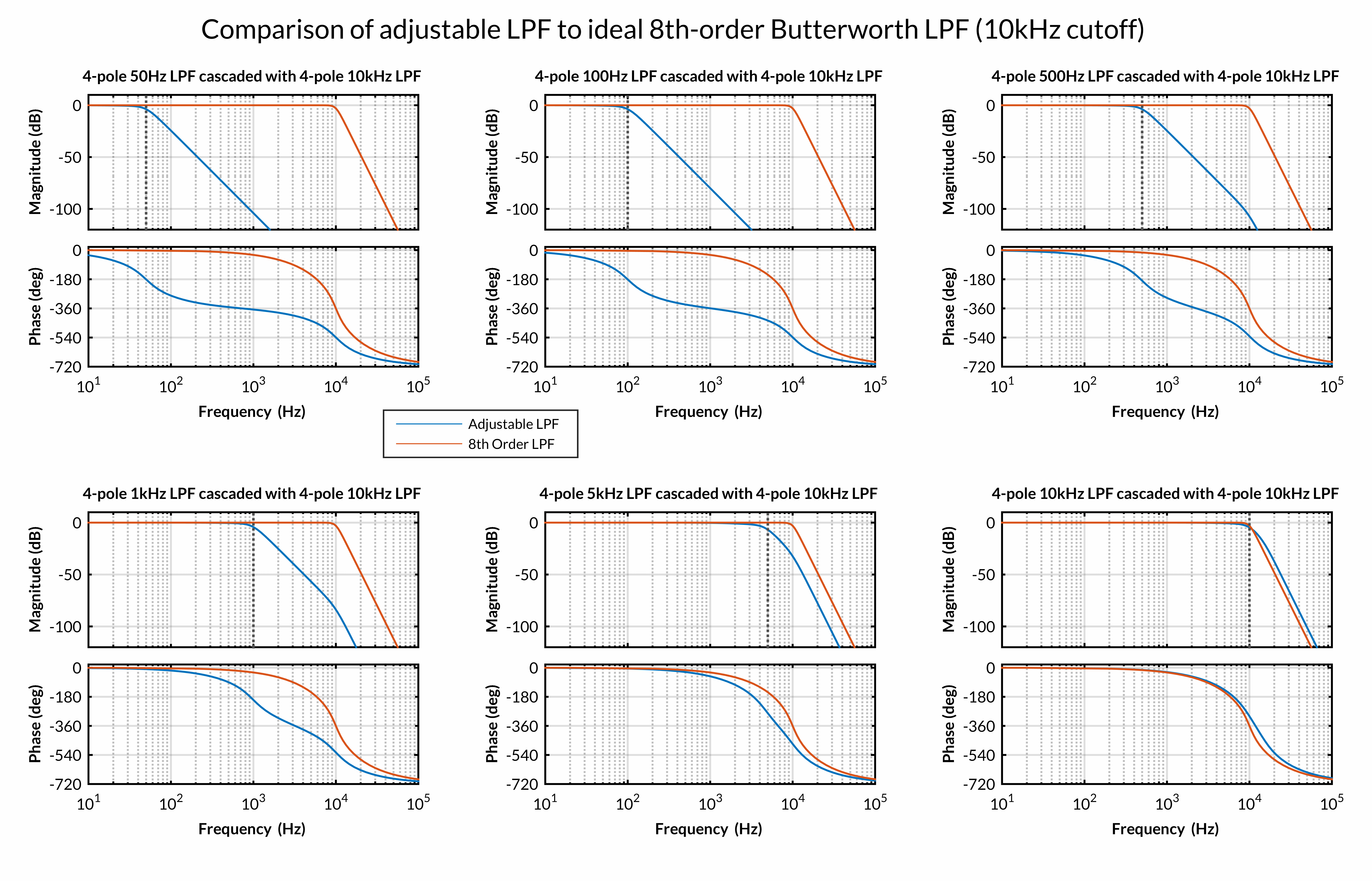
%% Compare filter realizations to ideal 8th order Sallen Key low pass filter with 10kHz-cutoff
RCfilter.transfer1234 = RCfilter.transfer12 * RCfilter.transfer34;

p = bodeoptions; p.FreqUnits = 'Hz'; p.XLim = [1,100000]; p.YLim = {[-120,10];[-720,20]};
% bodeplot(RCfilter.transfer1234(3),'k',RCideal.cascade,'r', p);

figure;
grid MINOR;

subplot(2,3,1);
bodeplot(RCfilter.transfer1234(1),RCideal.cascade, p);
title('4-pole 50Hz LPF cascaded with 4-pole 10kHz LPF');

subplot(2,3,2);
bodeplot(RCfilter.transfer1234(2),RCideal.cascade, p);
title('4-pole 100Hz LPF cascaded with 4-pole 10kHz LPF');

subplot(2,3,3);
bodeplot(RCfilter.transfer1234(3),RCideal.cascade, p);
title('4-pole 500Hz LPF cascaded with 4-pole 10kHz LPF');

subplot(2,3,4);
bodeplot(RCfilter.transfer1234(4),RCideal.cascade, p);
title('4-pole 1kHz LPF cascaded with 4-pole 10kHz LPF');

subplot(2,3,5);
bodeplot(RCfilter.transfer1234(5),RCideal.cascade, p);
title('4-pole 5kHz LPF cascaded with 4-pole 10kHz LPF');

subplot(2,3,6);
bodeplot(RCfilter.transfer1234(6),RCideal.cascade, p);
title('4-pole 10kHz LPF cascaded with 4-pole 10kHz LPF');

suptitle('Comparison of adjustable LPF to ideal 8th-order Butterworth LPF (10kHz cutoff)');
Section Output:RCfilter.transfer1234(1)= (1.532e29) / (s^8 + 1.656e05 s^7 + 1.368e10 s^6 + 6.632e14 s^5 + 1.625e19 s^4 + 1.377e22 s^3 + 5.558e24 s^2 + 1.343e27 s + 1.532e29) RCfilter.transfer1234(2)= (2.461e30) / (s^8 + 1.665e05 s^7 + 1.383e10 s^6 + 6.751e14 s^5 + 1.683e19 s^4 + 2.805e22 s^3 + 2.251e25 s^2 + 1.084e28 s + 2.461e30) RCfilter.transfer1234(3)= (1.502e33) / (s^8 + 1.733e05 s^7 + 1.499e10 s^6 + 7.733e14 s^5 + 2.175e19 s^4 + 1.581e23 s^3 + 5.986e26 s^2 + 1.37e30 s + 1.502e33) RCfilter.transfer1234(4)= (2.245e34) / (s^8 + 1.817e05 s^7 + 1.647e10 s^6 + 9.039e14 s^5 + 2.866e19 s^4 + 3.626e23 s^3 + 2.549e27 s^2 + 1.096e31 s + 2.245e34) RCfilter.transfer1234(5)= (8.393e36) / (s^8 + 2.377e05 s^7 + 2.817e10 s^6 + 2.127e15 s^5 + 1.085e20 s^4 + 3.706e24 s^3 + 8.537e28 s^2 + 1.243e33 s + 8.393e36) RCfilter.transfer1234(6)= (8.516e38) / (s^8 + 3.94e05 s^7 + 7.742e10 s^6 + 9.861e15 s^5 + 8.702e20 s^4 + 5.399e25 s^3 + 2.321e30 s^2 + 6.369e34 s + 8.516e38)
RFI_filter.m
%% RFI Filter Design
%
%                 GND
%                 |
%                 C1
%                 |       |\
%     -IN ----R---o-------|-\
%                 |       |  \
%                 C2      | IA ------ OUT
%                 |       |  /
%     +IN ----R---o-------|+/
%                 |       |/
%                 C1
%                 |
%                 GND

clc; clear all; close all;

R = 2200;
C1 = [1] * (10^-9);
C2 = [10] * (10^-9);

BW_diff = 1./(2*pi*R*(2*C2 + C1))
BW_cm = 1./(2*pi*R*C1)
Current Schematic
What's next?
- Further tweaks to the design
- PCB layout and etching
- Assembly
- Testing
- Software (work-in-progress; more details to be released as more of the project is finalized)
References
[1]: Cygnar, K. D., Stephan, A. B., Zhao, H. Analyzing Responses of Mouse Olfactory Sensory Neurons Using the Air-phase Electroolfactogram Recording. J. Vis. Exp. (37), e1850, doi:10.3791/1850 (2010).
To leave a comment below, sign in using Github.